Navigation: <-- Classification Tasks | Part Index | Main Index | Decision Trees -->

Classification Evaluation

Motivation: Your classifier reports 90% accuracy. That sounds good. But 90% of what? If 90% of examples in your dataset belong to the majority class, a model that always predicts "majority class" achieves 90% accuracy without learning a single pattern. So if accuracy is not the full story, how should we approach it?

In this nugget you'll learn to read a confusion matrix, derive precision, recall, and F1 from it, and match the right metric to the problem at hand. These tools apply to any classifier.

Interactive demo note: You can explore the behavior of all metrics in this nugget using the Classification Threshold & Metrics demo from my ✪ interactive data-science demos repository.

The Confusion Matrix

In 🖝 Classification Tasks, we introduced binary classification with positive and negative classes. For this scenario, each prediction falls into one of four cells:

	Predicted Positive	Predicted Negative
Actual Positive	True Positive (TP)	False Negative (FN)
Actual Negative	False Positive (FP)	True Negative (TN)

The definitions in detail:

True Positive (TP): the model predicted positive and was right = a correct detection.
True Negative (TN): the model predicted negative and was right = a correct dismissal.
False Positive (FP): the model predicted positive but was wrong = a false alarm.
False Negative (FN): the model predicted negative but missed a real case = a miss.

In the classification demo from ✪ interactive data-science demos you can also explore the confusion matrix and what it change while you adjust the threshold slider:

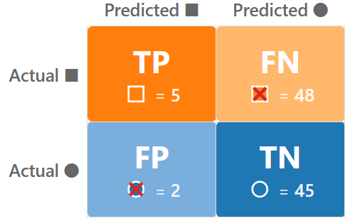
Tipp: A confusion matrix immediately reveals the potential pitfall of a classifier that just predicts the majority class (common for imbalanced classes). In the confusion matrix, one entire row will be empty or near-empty.

Precision, Recall, and F1: When Accuracy Is Not Enough

Introducing precision and recall

Class imbalance and assymetric error costs can be addressed by two complementary metrics. For these formulas we also use \(\text{P}\) and \(\text{P'}\) - the number of actual positives in the ground truth vs. the number of predicted positives.

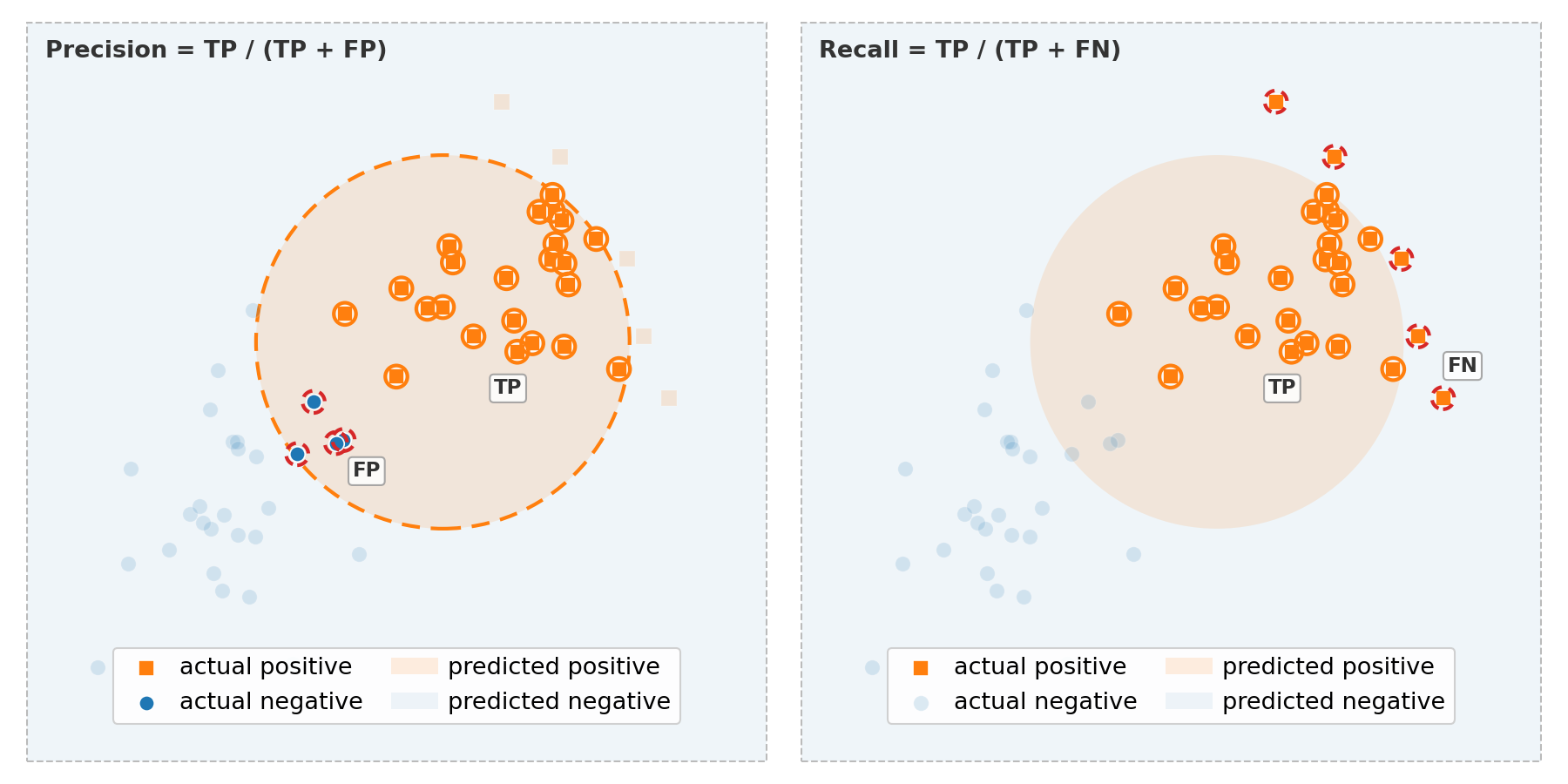
Precision answers: "Of all the records I predicted as positive, how many actually are?"

\[\text{Precision} = \frac{\text{TP}}{\text{P'}} = \frac{\text{TP}}{\text{TP} + \text{FP}}\]

Recall (also called sensitivity or true positive rate) answers: "Of all records that are actually positive, how many did I find?"

\[\text{Recall} = \frac{\text{TP}}{\text{P}} = \frac{\text{TP}}{\text{TP} + \text{FN}}\]

Here's an illustration of both metrics, using Venn diagrams:

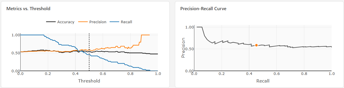
Precision-recall trade-off

Precision and recall together represent a trade-off:

You can always increase recall by predicting positive more aggressively, but then precision drops.
You can increase precision by predicting positive only when very confident, but then recall drops.

The trade-off can be seen via precision-recall curves (their behavior is best explored with the interactive demo):

F1 as a compromise between precision and recall

Next, F1 is the harmonic mean of precision and recall. It penalizes extreme imbalance between the two:

\[F1 = \frac{2 \cdot\text{Precision} \cdot \text{Recall}}{\text{Precision} + \text{Recall}}\]

A model with precision = 0.9 and recall = 0.1 gets \(F1 = 0.18\). In contrast, using arithmetic mean would give use a value of 0.5. Therefore, the harmonic mean penalizes strong discrepancy between precision and recall more, which is often desired. For example, a model that almost never fires for positives is seldomly useful.

Overview of all quantities

Finally, here's another view to build some intuition about the quantities that appear in the confusion matrix and the metric definitions. It shows how quantities flow into one another: from \(\text{Total}\) (all examples) → \(\text{P}\) and \(\text{N}\) (the number of actual positive/negative examples) → \(\text{TP}\), \(\text{FN}\), \(\text{FP}\), \(\text{TN}\) (the confusion matrix cells, red arrows indicate "error" paths) → \(\text{P'}\) and \(\text{N'}\) (the number of examples that where predicted as positve/negative) → \(\text{Total}\) again (all predictions).

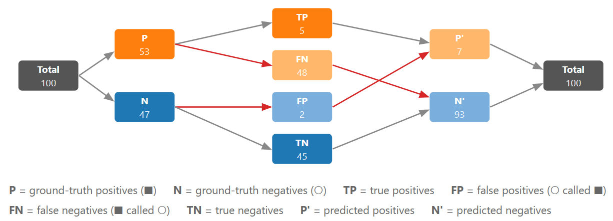
All Quantities and how they flow into each other

The left side in this diagram coresponds to the ground truth (actual labels) and the right side to "what the model predicts".

First Metric Choice: Matching the Metric to the Use Case

The right metric depends on the cost of each type of error in your specific application. We cover this in detail in 🖝 Choosing and Aligning Metrics. Here's an overview already:

When false negatives are more costly (missing a real case is worse than a false alarm): prioritize recall.

Examples: screening for a disease, flagging safety incidents.

When false positives are more costly (false alarms carry a high cost): prioritize precision.

Examples: spam filtering where legitimate email must not be lost.

When both error types carry similar cost and classes are roughly balanced: accuracy is a fair summary.

When both errors matter and classes are imbalanced: use F1.

Discussion: You build a model to predict whether a machine component is about to fail. Missing a failure (FN) causes expensive downtime and a safety risk. A false alarm (FP) triggers an unnecessary maintenance check costing a few hours. Which metric would you optimize for?

In real-world business applications, it is not uncommon to model the actual costs using the FN and FP rates of a model explicitly.

Summary

The confusion matrix shows the four outcome types for binary classification: TP, TN, FP, FN.
Accuracy is misleading when classes are imbalanced.
Precision measures the correctness of positive predictions. Recall measures the coverage of actual positives. F1 is their harmonic mean.
Choose your primary metric based on which type of error is more costly in your application.

As always: Happy learning, happy life! 🫶