Navigation: <-- Classification Evaluation | Part Index | Main Index | Random Forests -->
Decision Trees
Requires: Supervised Learning · Classification Evaluation
Motivation: The classifiers from 🖝 Classification Tasks turn a continuous score into a binary decision by applying a threshold. This was not yet end-to-end though: We left open where the scores come from. While we don't answer this question here, we want to introduce our first end-to-end classification model. We always want to start simple. So what about a model that you can read, audit, and explain to anyone?
In this nugget you will learn how a decision tree converts training data into if-then-else rules and how the best splits are chosen. You will also extend the evaluation tools from 🖝 Classification Evaluation to multi-class problems, where each class receives its own precision, recall, and F1 score. Finally, you will learn to interpret a trained tree and see why interpretability is the tree's defining strength.
Interactive demo note: You can try everything from this nugget using the Decision trees demo from my ✪ interactive data-science demos repository.
Table of Contents
- Decision Trees
- Multi-Class Evaluation
- Interpreting Trees
- Summary
- Bonus: Building the Tree
- References
Decision Trees
A decision tree is a flowchart. Each internal node tests one feature against a threshold. Each branch follows one outcome of that test. Each leaf assigns a class label via the leaf's majority class (so among the training examples that end in this leaf). To classify a new example, you walk from the root to a leaf, following the branches that match the example's feature values.
Let's take a look at an example. The Palmer Penguins dataset has three species (Adelie: blue, Chinstrap: orange, Gentoo: green), four features, and 333 samples. Here's a decision tree of depth 2 trained on the dataset. Colors in each node show the class proportions among the training examples that reached that node:
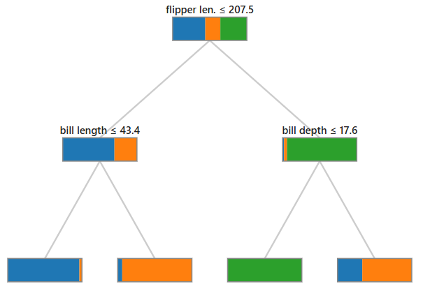
- The root splits on flipper length ≤ 207.5 mm: examples above the threshold flow right, the examples that land here are almost exclusively Gentoo.
- The right branch splits on bill depth ≤ 17.6 next, which perfectly separates the Gentoo class on the training data.
- The left branch splits on bill length ≤ 43.4, which separates Adelie from Chinstrap quite well.
We could train deeper trees to get even better results on the training data. However, this can lead to overfitting easily.
Overfitting pitfall: A fully grown tree memorizes the training set and generalizes poorly. So depth needs to be balanced.
To balance depth, several pruning strategies are available:
- either stop splitting early when the gain falls below a threshold, or
- grow the full tree and then remove branches that hurt held-out performance (post-pruning).
The simplest way to restrict maximum tree depth directly during fitting the tree.
When using scikit-learn DecisionTreeClassifier, all these options can be controlled via hyperparameters: max_depth, min_samples_leaf, and min_samples_split.
Discussion: You train a decision tree that achieves 98% training accuracy and 67% test accuracy. Your manager says: "We should deploy this: 98% is excellent." How do you explain the problem, and what would you do next?
See also: 🖝 Generalization.
Multi-Class Evaluation
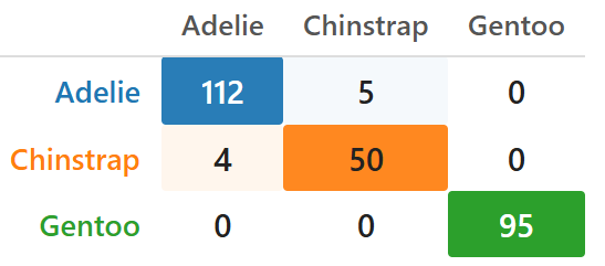
First of all, the concept of a confusion matrix from 🖝 Classification Evaluation generalizes straight-forward to a multi-class setting:
Now, let's take a look at the classification metrics. Up to this point, precision, recall, and F1 were defined for a binary problem with one positive class. Many real tasks have more than two classes: species, product categories, medical diagnoses. Decision trees handle multi-class problems natively, since leaves can predict any class, but evaluation needs to extend as well.
The key idea is straightforward: for each class, treat it as the positive class and all other classes as negative. This gives you a precision, recall, and F1 per class. Scikit-learn's classification_report does exactly this:
The report for the depth-2 penguins tree above is this (computed for test data, where we do evaluation):
| Class | Precision | Recall | F1 | n |
|---|---|---|---|---|
| Adelie | 0.97 | 0.97 | 0.97 | 29 |
| Chinstrap | 0.81 | 0.93 | 0.87 | 14 |
| Gentoo | 1.00 | 0.92 | 0.96 | 24 |
Chinstrap shows the weakest precision (0.81): some Adelie or Gentoo examples are misclassified as Chinstrap. This is expected given the depth-2 constraint, since the tree cannot separate Chinstrap perfectly with only two splits. Gentoo achieves perfect precision (1.00) because the "right-then-left" leaf is entirely Gentoo in the training data, though recall is slightly below 1 as a few Gentoo examples are still misclassified.
The column n counts actual examples of each class in the test set. Note: A class with few test examples (small n) gives an unreliable estimate of its metrics.
TODO: the other metrics in the report (not shown in table)...
Tip: The
macro avgrow averages the per-class metrics without weighting by class size. Theweighted avgweights byn. For imbalanced classes,weighted avgcan mask poor performance on minority classes, so keep both in view.
Interpreting Trees
Interpretability is the decision tree's defining strength. Follow any path from root to leaf and you have a complete, human-readable rule: "If flipper length is above 207.5 mm and bill depth is smaller than 17.6 mm, predict Gentoo." No formula needed, no statistical background required.
Three signals to read from a trained tree:
- The root split: The feature on which the split happens is often a strong global predictor.
- Leaf purity shows how confident each prediction is. A leaf where 95% of training records belong to one class is a confident predictor. A 55/45 split is close to a coin flip.
- Depth trades interpretability for expressiveness. Trees with depth roughly greater than three become harder to explain to an audience.
This shows that trees are simple models with good 🖝 Explainability properties. See also 🖝 Random Forests for how combining many trees addresses fragility, overfitting, and global feature importance.
Summary
- A decision tree classifies by recursively splitting on the feature and threshold that maximize information gain, producing a flowchart of if-then-else rules.
- For multi-class problems, precision, recall, and F1 are computed per class by treating each class as the positive class against all others. Scikit-learn's
classification_reportsummarizes this directly. - Interpretability is the decision tree's signature strength: each root-to-leaf path is a human-readable rule, and the root split identifies the feature with the highest information gain on the training data.
- Deep trees overfit. Depth-limiting and pruning are the primary remedies, and ensemble methods like random forests address the fragility of a single tree.
Bonus: Building the Tree
The standard recursive procedure is Hunt's Algorithm (Tan et al., 2020):
- If all training records at the current node belong to the same class, make that node a leaf.
- Otherwise, choose the feature and threshold that best separates the records and split. Distribute records to the child nodes accordingly.
- Repeat recursively for each child.
Here, "best" is defined by impurity. A pure node contains records from only one class. There are basically two measures that are commonly used: entropy and gini.
Information gain as impurity measure
The most interpretable measure is Shannon entropy:
where \(p_v(c)\) is the proportion of class \(c\) at node \(v\). Entropy measures how mixed a node is. A perfectly pure node has entropy \(0\): you always know the class, so there is no uncertainty. A node with equal proportions across all classes has maximum entropy: like a fair coin, the label is completely unpredictable.
The information gain of a split \(s\) measures how much it reduces uncertainty. Intuitively, it is entropy before the split minus the entropy remaining after the split:
Here, the sum runs over the child nodes \(v_j=v_j(s)\) produced by \(s\) from parent node \(v\), weighted by their fraction \(N(v_j)/N\) of the parent's data points. The second term is a size-weighted average of child entropies. A good split produces purer children, so that average is low and \(\Delta\) is large. A split that does not separate the classes leaves each child as mixed as the parent, and \(\Delta \approx 0\).
Ultimately, at each node, the algorithm selects the split with the highest information gain:
where \(s\) is a (feature, threshold) pair. The search is exhaustive: for each feature, every boundary between consecutive distinct values in the current node's records is a candidate threshold, giving a finite set of \(O(N \cdot k)\) candidates, where \(N\) is the number of records at the current node and \(k\) is the number of features.
Concrete example: suppose a parent node has \(N=10\) records, 5 of class A and 5 of class B, giving entropy \(1\). A perfect split sends all A records to the left child and all B records to the right. Both children are pure with entropy \(0\), so:
The split removed all uncertainty. Any less clean split yields a smaller \(\Delta\), and the algorithm will prefer this one.
Gini as impurity measure
Gini impurity measures the probability that a randomly chosen record from node \(v\) is incorrectly classified when labelled at random from the node's class distribution. Like entropy, it equals zero for a pure node and is maximal when all classes are equally represented. Splits are chosen by maximizing the weighted reduction in Gini across children. This is the same greedy principle as information gain:
Both entropy and gini select nearly identical splits in practice, so you can just use the default (Gini) from DecisionTreeClassifier.
In practice, Gini is slightly faster (no logarithm), entropy produces a sharper penalty on mixed nodes.
References
Tan, P.-N., Steinbach, M., Karpatne, A., & Kumar, V. (2020). Introduction to Data Mining (2nd ed.). Pearson.
As always: Happy learning, happy life! 🫶
Navigation: <-- Classification Evaluation | Part Index | Main Index | Random Forests -->
Script v1.4 (2026-06-10) · FGN