Navigation: <-- Transfer Learning | Part Index | Main Index | Transformers -->

Autoencoders

Requires: What Deep Networks Learn: Representations · Anomaly Detection

Motivation: In 🖝 Anomaly Detection and 🖝 Isolation Forests, you built anomaly detectors using statistical thresholds and tree-based isolation. These methods are mostly viable on tabular data with just a few features. However, if the input data is high-dimensional, like spectrums or large images, then neither "classical" method scales well. In those cases, autoencoders can bring the representational power of deep learning to anomaly detection.

In this nugget, you'll see how a network can be trained to reconstruct its own inputs, how to read high reconstruction error as anomaly signals, how the encoder-decoder architecture connects to the representation concepts from the previous nuggets. You'll generally see when autoencoders are the right tool compared to simpler baselines.

Interactive demo note: You can interactively explore everything from this nugget in the Autoencoder demo from my ✪ interactive data-science demos repository.

Reconstruction Error as an Anomaly Signal

An autoencoder (Hinton & Salakhutdinov, 2006) is a neural network trained to reproduce its own input. The network takes an input \(\mathbf{x}\), maps it to a compressed intermediate representation (the "latent" bottleneck), and then tries to reconstruct \(\hat{\mathbf{x}}\) from that representation. The loss function is the reconstruction error, which measures the discrepancy between \(\mathbf{x}\) and \(\hat{\mathbf{x}}\). A typical choice sums the squared deviations:

\[\mathcal{L} = \frac{1}{n} \sum_{i=1}^{n} \|\mathbf{x}_i - \hat{\mathbf{x}}_i\|^2.\]

The idea for autoencoders is that they should learn to compress and reconstruct the patterns typical of normal inputs.

When used for anomaly detection, autoencoders are trained on normal data only.

During inference (after training), a well-trained autoencoder then behaves as follows:

For normal inputs, the autoencoder produces small reconstruction errors - because the data is similar to what the autoencoder has seen during training.
For anomalous inputs (that look different from anything in the training set), the autoencoder cannot reconstruct them well, producing a high reconstruction error.

This is the anomaly signal: typical/normal inputs produce low reconstruction error; anomalous inputs produce high reconstruction error.

Like 🖝 Isolation Forests or other anomaly detection methods, the approach requires no anomaly labels. You only need a collection of normal examples, which is usually available: a machine running correctly, a product without defects, a system in steady state. This is a big advantage!

Note: To flag anomalies, some kind of threshold is needed to separate "high" from "low" reconstruction error. This threshold is a hyperparameter. You set it based on the distribution of reconstruction errors on a held-out normal set, just as you would set a z-score threshold in 🖝 Anomaly Detection. The threshold controls the tradeoff between precision (not raising too many false alamars) and recall (not missing real anomalies).

Connection to Deep Learning

An autoencoder consists of two subnetworks:

The encoder maps the input to a low-dimensional representation: \(\mathbf{z} = \text{Encoder}(\mathbf{x})\)
The decoder maps the representation back to the input space: \(\hat{\mathbf{x}} = \text{Decoder}(\mathbf{z})\)

The bottleneck ist the low-dimensional layer \(\mathbf{z}\) between encoder and decoder. This is exactly the embedding from 🖝 What Deep Networks Learn: Representations: Here, it is chosen relatively low-dimensional on purpose. It has no capacity to model noise from the input. Generally, the encoder is learning a compressed representation of the input.

For normal inputs, this representation captures the structure efficiently (though it may cut away "high-frequency features" like sharp edges).
For anomalous inputs, the bottleneck discards the unusual details, and reconstruction fails.

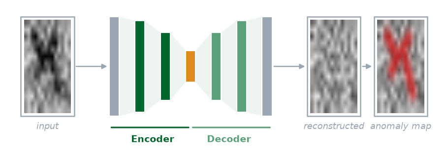
The encoder is also a feature extractor. The bottleneck \(\mathbf{z}\) tends to capture the most structure-relevant information in the input. Since it contains semantic information, the bottleneck can therefore be used for clustering, visualization (e.g., via t-SNE), or as input to a downstream classifier if some labels later become available. This dual use, anomaly detection and representation learning, makes autoencoders a flexible building block.

When to Consider Autoencoders

Nevertheless, an autoencoder is not always the right tool. Simpler methods should come first. The principle from 🖝 Baselines and the Good-Enough Bar applies here exactly as elsewhere: start with z-score thresholds from 🖝 Anomaly Detection, then try 🖝 Isolation Forests, unless the data domain prohibits it outright due to high-dimensionality.

Here's an overview of conditions that favor autoencoders:

High-dimensional input: images, spectra, waveforms with hundreds/thousands of channels.
Enough normal training data: Autoencoders need enough examples of normal behavior to learn a good reconstruction model. A few dozen examples are usually not enough, while a few hundred to a few thousand can provide a more robust training ground.
Compute budget allows it: an autoencoder is more expensive to train and serve than a the "classical" methods (such as thresholds or isolation forests). For real-time embedded systems, this cost may be prohibitive.

Discussion (mini "case study"): An autoencoder trained on spectroscopy data from a chemical process flags a sample as anomalous (high reconstruction error). A domain expert inspects the sample and says it looks normal to them. Is this more likely to be a true false positive, a threshold calibration issue, or a sign that the autoencoder learned spurious patterns in the training data? How would you investigate each of these possibilities?

Summary

Autoencoders are trained to reconstruct inputs. Trained on normal data only, it reconstructs normal inputs well and anomalous inputs poorly. High reconstruction error is the anomaly signal.
The encoder-decoder structure produces a bottleneck embedding, connecting autoencoders directly to the representation learning concepts (previous nugget).
Autoencoders are the right tool when inputs are high-dimensional (images, spectra), enough normal data is available for training, and simpler baselines are insufficient.

As always: Happy learning, happy life! 🫶