Navigation: <-- Transformers | Part Index | Main Index | Part IX: Closing the Loop - Projects in Practice -->

Deep Learning in Practice: Choosing and Applying

Requires: Convolutional Neural Networks (CNNs) · Transfer Learning · Autoencoders · Start Simple

Motivation: This part has introduced deep networks, CNNs, representations, transfer learning, autoencoders, and transformers. When do you reach for any of them, and how do you set up the work? Deep learning is not inherently better than the methods from 🖝 Part V: Supervised Learning to 🖝 Part VII: Unsupervised Learning. It is appropriate for specific problems and introduces specific costs. This nugget gives you the decision framework to navigate that.

You'll get a structured approach: starting from the problem rather than the method, checking whether DL is actually warranted, choosing the right architecture family, and setting up the training pipeline.

Work Problem-Centric

Every method decision should start from the task, not the toolbox. "We want to use a transformer" is not a good start for a project, which requires a good definition of problem and goals. "We have maintenance reports in free text and want to classify them by fault type" is better, and may just happen to suggest a transformer.

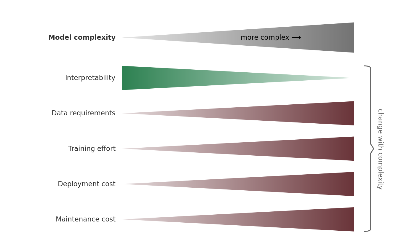
The principle from 🖝 Start Simple applies here fully. Deep learning is not simple. It adds data requirements, compute requirements, longer iteration cycles, and interpretability costs. If 🖝 Random Forests or 🖝 Logistic Regression already solve the problem, use either of them. Deep learning is worth its cost only when simpler methods genuinely are no match.

The right sequence:

Define the problem, prediction target, and success criterion.
Establish a baseline (majority class, mean predictor, simple threshold).
Try the simplest appropriate model for your input type.
Only escalate to deep learning if the gap to the required performance is real and the constraints (below) allow it.

Note: The common sense "deep learning probably works best here" still warrants step 3: Knowing the gap is helpful, and simpler models often surprise.

Check the Constraints

Before committing to a deep learning approach, audit these constraints:

Data volume and quality: DL needs substantial labeled data. 🖝 Transfer Learning lowers the bar; training from scratch needs far more. Too little data means overfitting, in this case, simpler methods usually generalize better.
Compute budget: Training cost ranges from a few accessible GPU-hours (CNNs, fine-tuned models) to far more (a large language model). Know what's realistic.
Interpretability requirements: Deep network performance is the hardest to explain to stakeholders or regulators. Post-hoc tools like SHAP (see 🖝 Explainability) help but only approximate. Simpler models are transparent by construction.
Latency: Check inference time against the deployment target, e.g., a production line running at 10 parts per second. Simpler models are almost always faster.
Maintenance cost: DL pipelines need more infrastructure, GPU serving, model versioning, drift monitoring, retraining.

To complete the picture, here's our figure from 🖝 Start Simple again:

Choose the Model Family

Given that DL is warranted, which architecture? The input modality drives the choice more than any other factor:

2D images: CNN + transfer learning. Use a pretrained backbone (ResNet, EfficientNet); train from scratch only with large labeled datasets. See 🖝 Convolutional Neural Networks (CNNs) and 🖝 Transfer Learning.
Text, NLP: pretrained transformers, consider to fine-tune on your task data. See 🖝 Transformers.
Audio / time-series: 1D CNN for short local patterns, Transformer for long-range or cross-position dependencies. See 🖝 Convolutional Neural Networks (CNNs) and 🖝 Transformers.
Unlabeled anomalies, high-dim data: autoencoders, when simpler baselines like 🖝 Isolation Forests fail on images, spectra, or complex waveforms. See 🖝 Autoencoders.
Tabular data: tree-based methods first. Deep learning rarely outperforms gradient boosting at the same data size. See 🖝 Random Forests.

All these suggestions are just starting points that can be overriden by domain knowledge, data volume, and the specific task.

See also: 🖝 When Shallow Models Fail.

Build the Training Loop

Once the architecture is chosen, training needs to be set up. Typical mistakes here include data leakage, improper normalization, or evaluation the wrong way. Such mistakes will invalidate results regardless of architectural choices. To avoid such mistakes, some key aspects to consider are:

Preprocessing: normalize inputs to what the architecture expects, pixel scaling for images, the pretrained model's own tokenizer for text, raw waveform vs. spectrogram for signals.
Dataset loaders and batching: data is read and fed to training in mini-batches; batch size trades gradient stability (larger) against memory cost and a regularizing noise effect (smaller).
Data augmentation: input-preserving transforms (crops, flips, jitter for images; time-shifting for signals; synonym swaps for text) that act as regularization by expanding the effective dataset.
Splits and evaluation pipeline: split into train/validation/test before computing any statistics from the data (normalization, augmentation ranges), and touch the test set only once, at the end.
Iterative error analysis: after each iteration, inspect which validation examples fail and why, then fix the most impactful source of error before adding model complexity.

Warning: A common source of silently wrong results in deep learning is data leakage: test images appearing in the training set, or normalization statistics computed on the full dataset before splitting, see 🖝 Data Splits.

Summary

Start from the problem, not the method.
Before committing to DL, check constraints: data volume, compute budget, interpretability requirements, latency, and maintenance cost.
Input modality drives architecture choice.
Set up the training loop carefully: split before normalizing, apply augmentation as regularization, monitor validation with early stopping, and use iterative error analysis.

As always: Happy learning, happy life! 🫶